A Detailed Look at Confidence Interval

Photo by NASA on Unsplash

Stats had always been a subject that I found so abstract to comprehend. However, it is one of the most import building blocks of Data Science and Machine Learning. With the increasingly accessible computing power and availability of advanced packages for statistical analysis, one could probably perform a data analysis and build a model fairly quickly without having a thorough understanding of the key statistical concepts. But I would argue that it will likely not be a good one. And most importantly, it will probably lack interpretability to drive real business values, which is the ultimate goal of most data science projects.

One of the fundamental concepts in statistics is Confidence Interval. Most people including myself have learned about it in our undergrad stats course and the formula for calculating a Confidence Interval. But at the beginning, I always found myself perplexed by phrases such as ‘We are 95% confident about this value’. I want to therefore do a simple review on this topic.

Background Info

Before I get into what confidence interval is used for, there are some important concepts to keep in mind:

• Parameter: a summary measure of characteristic of the entire population. (i.e. population mean)
• Statistic: a summary measure of characteristics of a sample data. (i.e. sample mean)
• Statistical Inference: the process of using observed sample data to learn about a population of interest. This can generally be divided into Estimation and Hypothesis Testing.
• Estimation: a procedure for using a statistic to estimate the value of a unknown population parameter.
• Hypothesis Testing: a procedure for using a statistic to evaluate claims about the unknown population parameter.
• In data analysis, Estimation often follows Hypothesis Testing. For example, suppose a hypothesis test found evidence that a parameter is greater than 50. Your next goal would likely be to estimate how much greater than 50 it is.
• Sampling Variability: information about a population varies depending on which of the possible samples was selected. In the example below, all 4 samples come from the same population with a population mean of 0 and a population standard deviation of 1. But the value of a statistic varies from sample-to-sample:

4 samples with different means and standard deviations

• CLT (Central Limit Theorem): for sufficiently large samples, the sample mean (X̄) will be normally distributed with the mean (µ) and standard deviation (σ/√n), where µ is the population mean, σ is the population standard deviation, and n is the sampe size. Mathematically, this can be written as:

Motivation

When conducting data analysis or a research, we might ask questions like what is the average birth weight of all babies born in 2020 in California? Or we could be interested in finding out the average vote turnout rate in an election campaign across North Carolina. These type of questions all fall under the umbrella of quantity estimation, where the goal is to estimate a population parameter in interest. And there are generally two ways to go about it:

1. Point Estimate: this can be seem as using the ‘best guess’ to estimate the population parameter based on one observed sample. Using the turnout rate as an example, we might observed that the turnout rate in Durham County was 0.67 and decided to use that as the turnout rate for all North Carolina. However, it is very unlikely that this point estimate accurately represents the turnout rate for the entire state, because it did not take sampling variability into consideration.
2. Confidence Interval (Interval Estimate): instead of giving a definite point estimate, confidence interval provides a range of plausible values, which is more likely to capture the true value of population parameter. Its biggest advantage over point estimate is that it accounts for sampling variability, which is inevitable in almost all real-life problems.

How It Works

Suppose we have a population with a mean blood sugar level of 100 mg/dl and a standard deviation of 20. I will use µ and σ to denote population average blood sugar level and standard deviation, respectively. Using CLT, we can say that the distribution of the sample mean for a sample size of 100 will follow a normal distribution with a mean of 100 and a standard deviation of 2 (that is , σ/√n = 20/√100). This distribution is illustrated in the figure below:

Conveniently, normal distribution has the following properties which could help us better interpret our sampling distribution.

For any normal distribution:

• ~ 68% of all possible values fall within 1 standard deviation of the mean.
• ~ 95% of all possible values fall within 2 standard deviation of the mean.
• ~ 99.7% of all possible values fall within 3 standard deviation of the mean.

This is called the empirical rule and is also shown in the following figure:

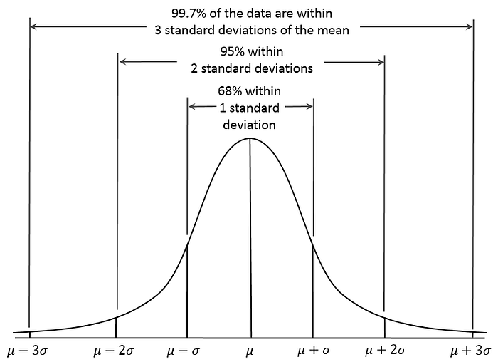
Utilizing this information, we can say that the probability that µ is within 2 standard deviations of the population mean is 0.95. In other words, we expect about 95% of the sample means to be between 96 mg/dl and 104 mg/dl.

This idea is captured in the following formulas, where the first part solves for the estimated range of the sample mean. However, we could easily transform it and solve for population mean instead.

So what we just produced was a 95% Confidence Interval for µ. What it means is that we are 95% confident that this interval captures the true value of population average blood sugar level, which is 100 mg/dl.

Now, suppose we took a random sample of 100 from this population and we determined the sample mean and standard deviation to be 97 and 16, respectively. Then, a point estimate for µ would be 97. And a 95% Confidence Interval for it would be (93.8, 100.2). In this case, our Confidence Interval successfully captured the true µ even though the point estimate clearly missed it. One thing to note is that for this hypothetical scenario, we knew what the µ is, and we can be sure that it’s within our Confidence Interval. However, this is rarely the case in real life. We say we are 95% confident because we only had access to the sample data. And depending on the sample, there is a chance that our Confidence Interval will miss the true value of µ.

The percentage in our Confidence Interval represents the confidence level of the interval estimate and could theoretically range from 0.01 to 0.99. However, we normally want to limit it to between 0.90 and 0.99 for high confidence.

Interpretation of CI

After we determine a 95% Confidence Interval, we could say that we are 95% confident that the interval captures the true value of the population parameter. But what does it mean when we put a quantity on confidence?

In the previous section, we mentioned that albeit a low probability, there is a chance our constructed Confidence Interval could miss the true population parameter. Going back to the blood sugar level example, if the sample mean was 96 instead, then our Confidence Interval would be (92.8, 99.2). This interval estimate would have missed the true value of µ. And this is the reality of sampled-based research and inference.

Therefore, the correct interpretation of a Confidence Interval is that — the true value of the population parameter will lie within the interval in 95% of similarly constructed Confidence Interval. This can be better visualized in the figure below using 20 random samples from the population:

In this figure, we expect 1 out of 20 confidence intervals (that is, 5%) to miss the true value of the population parameter.

What Influences CI

I don’t intend to go through the math part. But if you work out the formula above and understand what I have reviewed so far, then it’s pretty straightforward to see that there are two things that could influence the width of a Confidence Interval besides sample standard deviation:

• Confidence Level: the higher the confidence level, the wider the width. (i.e a 99% Confidence Interval is wider than a 90% Confidence Interval)
• Sample Size: the larger the sample size, the more confident we are, therefore the narrower the width. (i.e a 95% Confidence Interval produced from a sample size of 100 observations is narrower than that produced from 50 observations)

Summary

In this post, I covered a pretty detailed review of Confidence Interval. Some key points are:

• A Confidence Interval an inference method used to estimate the population parameter such as population mean.
• It can be calculated from sample mean, sample standard deviation and sample size.
• Confidence level can range from 0 to 1, but we generally prefer 0.9+ for high confidence.
• The width of a Confidence Interval depends on confidence level and sample size.

The R script for producing the sample variability demo and normal curve can be found here. I hope this post can be useful for anyone who’s not super familiar with stats.