Simple Convolutional Neural Network with SHAP
CNN (Convolutional Neural Network) has been at the forefront for image classification. Many state-of-the-art CNN architectures had been devised in the recent years to tackle the hardest computer vision problem, range from digit classification to real-time object detection. In this blog, I will cover a simple convolutional neural network that can correctly identify image of bugs. Additionally, the applications of deep learning in many areas such as healthcare had always been controversial due to massive number of parameters and lack of interpretability. Much effort have been devoted in the area of interpretable neural network, one of which utilizes the Shapley Additive Explanation (SHAP). Therefore, I will also be exploring SHAP on my model.
Tools
The two most common packages for implementing neural networks are PyTorch and TensorFlow. For the purpose of this blog, I will be using PyTorch. However, the same architecture and training process could easily be implemented with TensorFlow.
In addition, I will be using SHAP package to explore Shapley values on the trained model.
Data
The dataset used for this project contains images of 3 different types of insects: beetles, cockroaches and dragonflies. There are 1019 training images in total, which consists of 460 beetles, 240 cockroaches, and 319 dragonflies. The validation dataset consists of 60 images of each insects. The following figure contains 10 sample images (resized):

The original data can be found on InsectImages.org.
Data Loading and Transformation
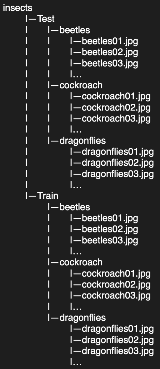
The first step is to load the data into the proper format (Batches) so it can be processed by a model properly. PyTorch torchvision has a built-in method ImageFolder that allows user to ingest data from the file system. This method requires the file system to be organized in the following way.:

In addition, this method allows user to perform any visual transformations such as resizing to all images contained in a dataset. To perform a series of transformation together, I use the transforms.Compose function, which accepts a list of transformations. This is illustrated in the following code snippet:
In the code above, the first transformation standardizes the size of all images to 224 x 224. The second transformation converts images to tensors, which is a required step for tensor manipulation in later stages. The final transformation normalizes each one of the RGB channels across all pixels of all images. Note that normalization requires prior knowledge on the mean and standard deviation values.
Next, I use PyTorch DataLoader to chunk data into batches of self-defined sizes (64 in this case). This step is needed for performing batch gradient decent, in which the neural network weights are updated based on a small batch of data as opposed to the entire training data, which significantly speeds up the training process. Note that shuffle is set to True for training data only:
Model Construction
For this project, I will use a simple architecture that consists of 2 convolutional layers and 3 fully connected layers. A max pooling layer and a batch normalization layer are after each convolutional layer, and the output is then fed into a ReLU activation function. The first convolutional layer uses a kernel size of 5 and the second one uses a kernel size of 3.
Before proceeding to the fully connected layer, I will need to first flatten the output of the convolution layers. Since the last convolution layer produced 16 by 54 by 54 tensor, I will flatten it using the .view method. Finally, the fully connected layers have an output size of 120, 84 and 3 respectively. Note that the size of the last fully connected layer needs to match the number of classes. The architecture’s PyTorch implementation is shown in the following snippet:
Training and Results
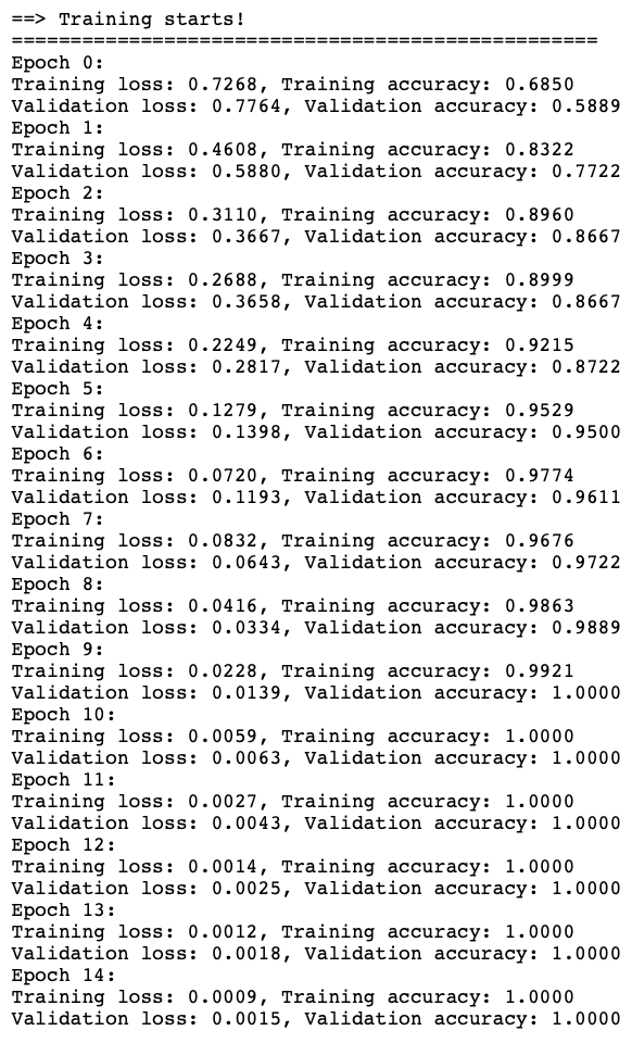
There are couple of things that need to be defined to train the model. The first one is the loss function, which in this case will be a Cross Entropy Loss XXX. For the gradient decent optimizer, I will use Stochastic gradient decent, with a learning rate of 0.01, a momentum of 0.9 and a weight decay of 1e-3. Using these hyper parameters, I’m able to get an accuracy of 100% within 15 epochs, as shown below:

The loss and accuracy over time are also plotted:

It can be seen that both the validation and training accuracy reached 100% at around the 10th epoch, which is also where the losses are minimized. This indicates that the constructed model is able to perfectly classify insects in the validation dataset.
SHAP
Shapley value is a concept from game theory. When applied to machine learning, the game is a prediction and each player is a feature. Therefore, the game payoff can be interpreted as the difference between the predicted value and the mean prediction where no features are used. In a nutshell, Shapley value provides an additive measure of feature importance. In the context of an image, each pixel is treated as a feature, therefore, Shapley value can be used to determine the pixel level importance in classifying images. This idea is illustrated in the figure blow:

The complete implementation can be found in this notebook:
